RAS598 • Fall 2024 • Machine Learning

Fashion MNIST
Classification

A comprehensive machine learning pipeline comparing deep learning models (CNN, ResNet) with traditional methods for classifying fashion items into 10 categories with 91% accuracy.

91% Accuracy
10 Classes
70K Images
7 Models

About The Project

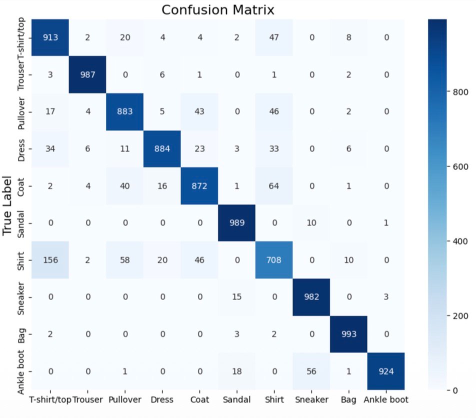
This research project explores the application of machine learning techniques to the Fashion MNIST dataset, focusing on classifying 28×28 grayscale images of fashion items into ten distinct categories including T-shirts, trousers, pullovers, dresses, coats, sandals, shirts, sneakers, bags, and ankle boots.

The project implements a comprehensive ML pipeline comparing deep learning architectures (CNN and ResNet) with traditional methods such as Logistic Regression, SVM, and Random Forest. Preprocessing steps including normalization and data reshaping were employed to optimize model performance.

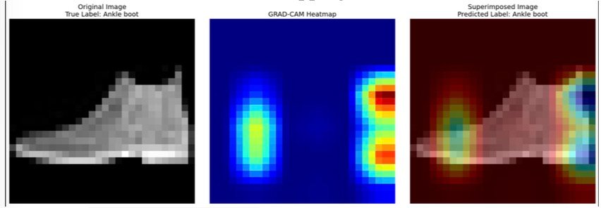
Grad-CAM visualizations enhance the interpretability of CNN predictions, building trust in model decisions for real-world applications in e-commerce, fashion retail, and manufacturing.

Python TensorFlow Keras Scikit-learn NumPy Matplotlib Seaborn Plotly
# Load Fashion MNIST dataset from tensorflow.keras.datasets import fashion_mnist (X_train, y_train), (X_test, y_test) = fashion_mnist.load_data() # Preprocessing X_train_cnn = X_train.reshape(-1, 28, 28, 1) / 255.0 X_test_cnn = X_test.reshape(-1, 28, 28, 1) / 255.0 class_names = ['T-shirt/top', 'Trouser', 'Pullover', 'Dress', 'Coat', 'Sandal', 'Shirt', 'Sneaker', 'Bag', 'Ankle boot'] # Training: 60,000 | Test: 10,000 # Image size: 28×28 pixels

Models Implemented

🧠

ResNet

Deep learning model utilizing residual connections to address vanishing gradient issues, enabling deeper architectures with robust generalization.

91%
🔮

CNN

Extracts spatial features from images using convolutional and pooling layers for high accuracy image classification tasks.

91%
🌲

Random Forest

An ensemble method aggregating decision trees, providing reasonable performance on flattened image data.

89%
📊

SVM

Employs kernel methods for non-linear classification, computationally expensive but effective for complex patterns.

87%
🔗

MLP

A fully connected neural network, limited in performance due to lack of spatial awareness in image data.

85%
📈

Logistic Regression

A simple linear classifier used as a baseline, limited in handling complex image patterns.

83%

Results & Analysis

Confusion Matrix

ResNet Model
Confusion Matrix showing classification results across 10 fashion categories

Classification Report

Per-Class Metrics
Class Precision Recall F1-Score
T-shirt/top 0.81 0.91 0.86
Trouser 0.98 0.99 0.98
Pullover 0.87 0.88 0.88
Dress 0.95 0.88 0.91
Coat 0.88 0.87 0.88
Sandal 0.96 0.99 0.97
Shirt 0.79 0.71 0.74
Sneaker 0.94 0.98 0.96
Bag 0.97 0.99 0.98
Ankle boot 1.00 0.92 0.96

Grad-CAM Visualization

Grad-CAM visualization showing model attention on ankle boot image

Understanding Model Decisions

  • 1
    Original Image
    The grayscale input image of an ankle boot used for classification.
  • 2
    Grad-CAM Heatmap
    Highlights regions most influential for the prediction. Bright areas (yellow/red) show model focus.
  • 3
    Superimposed View
    Combined visualization confirms the model correctly focuses on the shoe region for accurate prediction.

Future Work

🎨

Colored Image Support

Extend models to handle RGB images with complex backgrounds for improved real-world applicability.

🔍

Class-Specific Improvements

Address misclassifications between similar items like T-shirts and Shirts through targeted training.

🔀

Hybrid Models

Explore combinations of traditional and deep learning techniques for enhanced accuracy and efficiency.

Project Resources

📄

Project Report

Complete documentation including methodology, results, and analysis.

📊

Presentation Slides

Final project presentation with key findings and visualizations.

💻

Source Code

Complete Python implementation with CNN, ResNet, and traditional ML models.

Source Code

resnet_model.py
from tensorflow.keras import layers, models, optimizers def resnet_block(input_data, filters, conv_size): x = layers.Conv2D(filters, conv_size, activation='relu', padding='same')(input_data) x = layers.BatchNormalization()(x) x = layers.Conv2D(filters, conv_size, activation=None, padding='same')(x) x = layers.BatchNormalization()(x) x = layers.Add()([x, input_data]) x = layers.Activation('relu')(x) return x # Build ResNet Architecture input_layer = layers.Input(shape=(28, 28, 1)) x = layers.Conv2D(32, 3, activation='relu')(input_layer) x = layers.MaxPooling2D(2)(x) x = resnet_block(x, 32, 3) x = layers.MaxPooling2D(2)(x) x = resnet_block(x, 32, 3) x = layers.GlobalAveragePooling2D()(x) x = layers.Flatten()(x) output_layer = layers.Dense(10, activation='softmax')(x) resnet_model = models.Model(inputs=input_layer, outputs=output_layer)
cnn_model.py
from tensorflow.keras.models import Sequential from tensorflow.keras.layers import Conv2D, MaxPooling2D, Flatten, Dense, Dropout # Build CNN Architecture cnn_model = Sequential([ Conv2D(32, (3, 3), activation='relu', input_shape=(28, 28, 1)), MaxPooling2D((2, 2)), Conv2D(64, (3, 3), activation='relu'), MaxPooling2D((2, 2)), Conv2D(128, (3, 3), activation='relu'), Flatten(), Dense(128, activation='relu'), Dropout(0.5), Dense(10, activation='softmax') ]) cnn_model.compile( optimizer='adam', loss='sparse_categorical_crossentropy', metrics=['accuracy'] )
train.py
import numpy as np from tensorflow.keras.datasets import fashion_mnist # Load the Fashion MNIST dataset (X_train, y_train), (X_test, y_test) = fashion_mnist.load_data() # Preprocessing X_train_cnn = X_train.reshape(-1, 28, 28, 1) / 255.0 X_test_cnn = X_test.reshape(-1, 28, 28, 1) / 255.0 # Compile ResNet model resnet_model.compile( optimizer=optimizers.Adam(learning_rate=0.001), loss='sparse_categorical_crossentropy', metrics=['accuracy'] ) # Train the model history_resnet = resnet_model.fit( X_train_cnn, y_train, epochs=20, validation_data=(X_test_cnn, y_test) ) # Final Results: # Training Accuracy: 95% | Validation Accuracy: 91% # Training Loss: 0.1 | Validation Loss: 0.3
evaluate.py
from sklearn.metrics import confusion_matrix, classification_report import seaborn as sns import matplotlib.pyplot as plt class_names = ['T-shirt/top', 'Trouser', 'Pullover', 'Dress', 'Coat', 'Sandal', 'Shirt', 'Sneaker', 'Bag', 'Ankle boot'] # Predict on test data y_pred_resnet = np.argmax(resnet_model.predict(X_test_cnn), axis=1) # Compute confusion matrix cm = confusion_matrix(y_test, y_pred_resnet) # Plot confusion matrix using Seaborn heatmap plt.figure(figsize=(10, 8)) sns.heatmap(cm, annot=True, fmt='d', cmap='Blues', xticklabels=class_names, yticklabels=class_names) plt.title('Confusion Matrix', fontsize=16) plt.xlabel('Predicted Label', fontsize=14) plt.ylabel('True Label', fontsize=14) plt.show() # Classification Report print(classification_report(y_test, y_pred_resnet, target_names=class_names))

Meet The Team

KA

Karan Athrey

AS

Abhijit Sinha

AC

Anusha Chatterjee